

Natalie Fedorenko
Web analyst at PROANALYTICS.TEAMData-driven Attribution and Hands-On Practical Experience
Let’s start this article with a disclaimer: in addition to the technical and objective side — definitions, explanations of model principles, etc. — the text I’m offering you to read will also contain my subjective thoughts.
So, today’s agenda is packed:
Why I wrote this article
Sharing experience, as stated in the title of this article, is not my only goal. In addition, I also want to prompt you toward certain reflections and, perhaps, try to clear away the fog of mysterious complexity surrounding what is commonly called data-driven attribution. Sometimes, when talking to clients who are interested in something like this, it seems to me that the “data-driven” prefix adds a kind of “expert-level expertise” to decisions based on such attribution. It feels like we’ve already gotten used to the idea that decisions must be “data-driven,” meaning “based on data.” And I support that — but it should be approached critically, not mindlessly.
At the same time, unfortunately, people rarely realize the limitations of such models and the requirements that must be met for a model to truly deliver valuable insights rather than quietly mislead. So much positive has already been said about “data-driven” attribution that it can start to seem like this model is the only correct one for everyone without exception. However, not everyone can “afford” it, since, like any machine learning–based model, it requires consistent data in sufficient volume. Without meeting this condition, you will still get “data-driven” results, but with a high probability they will be far from the truth — something the model, of course, won’t tell you. At best, it will leave you alone with the question: “Can I trust these results and make important business decisions based on them?”
As for data consistency — it is crucial not to forget to properly tag your traffic so you can see the impact of the relevant channels. I recommend reading this article about proper tagging principles, where you can also get a UTM tagging template from our team.
What Is Data-Driven Attribution
Usually, you can read that data-driven attribution (DDA) is the most advanced model for distributing the value of a conversion across different touchpoints (channels) a user interacted with before making a purchase. But in reality, it is not a single model — it is a principle of value distribution.
There are two principles:
- rule-based
- and data-driven.
The difference lies in when the conversion value distribution coefficients are known. In the rule-based principle, they are known before the model is applied. These include models such as:
- last non-direct click — 100% of the value is assigned to the last known source before the conversion,
- linear distribution — all sources that participated in achieving the conversion receive an equal share of that conversion,
- position-based — the first and last sources receive 40% of the value each, and the remaining 20% is evenly distributed among the middle ones,
- time-decay — the closer a source is to the conversion, the larger share of the value it receives,
- first click — the entire value is attributed to the source of the first or first non-direct click to the website or app within the attribution window*.
*In addition to this definition, you may also encounter the interpretation that it is the source of the very first visit to the website or app. However, an important feature of all models is the presence of an attribution window — that is, the period before the conversion — and all touches that occurred within that period. Traditionally, attribution models are calculated within a 30- or 90-day window before the conversion. At the same time, the period can be any length — it all depends on how much time your potential customer needs to decide to convert and on your decision regarding the period during which, in your opinion, interactions with your offer could have influenced that customer’s acquisition.
All of these rules are not dependent on data and are the same for everyone implementing such an approach.
The data-driven principle lies in the fact that the model itself determines the value distribution coefficients during the learning process based on the data provided to it. Thus, these coefficients are unique for each model, and they can (and, in fact, should be able to) change over time even within the same project. Therefore, for DDA, the quality and sufficient volume of data are critically important, because they determine the value distribution and all the advantages that such an approach may have compared to rule-based models. “May,” but not necessarily “will.”

Which Data-Driven Model Is Used in GA4
I don’t know :)
That is, I cannot say which specific machine learning model DDA in GA4 is based on. The documentation “speaks” in general terms, such as:
“Data-driven attribution methodology includes two main stages:
- analysis of available data on paths to key events and development of conversion coefficient models for each key event;
- using the predicted key event conversion coefficient model outputs as input for an algorithm that assigns a percentage of value to different ad interactions.”
Below that, it provides an example that looks very similar to the Shapley value principle, which we will discuss later. Here, in the screenshot, chains with and without the Display channel are compared:
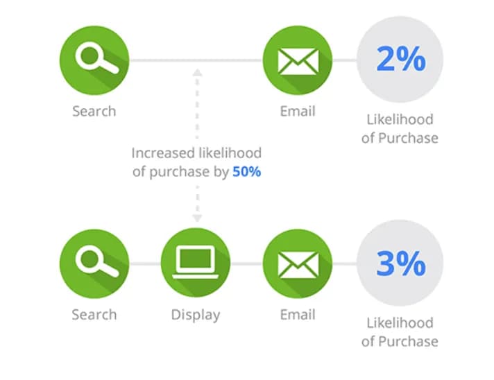
This example shows that chains that included the Display channel had a conversion rate of 3%, and if it was not present, the rate was 2%. Thus, the presence of the Display channel in the chain increases the probability of conversion by 50%.
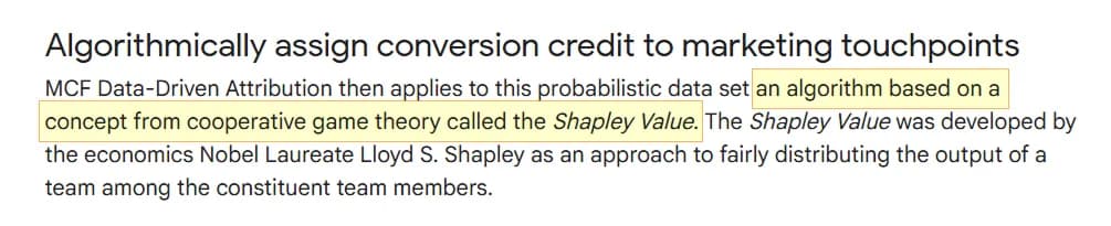
The assumption that GA4 uses the Shapley value as its foundation can be made based on deductive reasoning — in this help article it is explicitly stated that Google takes the Shapley value as a basis, with the note that “this feature is available only in Google Analytics 360.”
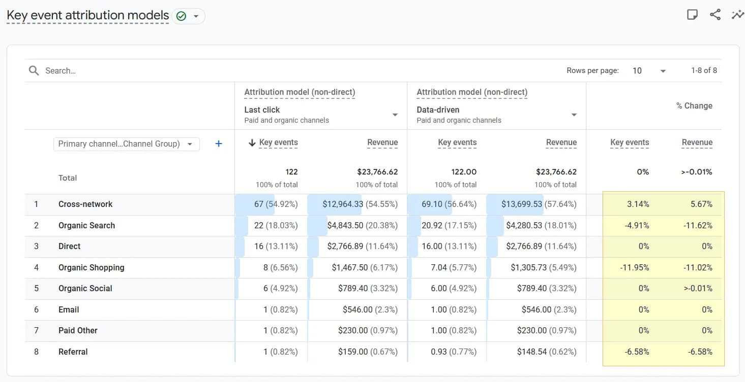
You will also see that the same approach was used in Universal Analytics. Personally, I doubt that standard Google Analytics uses something radically different in principle. Unless, perhaps, it is an improved version that does not account for direct traffic in chains, as indicated by the “non-direct” prefix next to the names of all the models that remain in GA4.

And we are saying that the Shapley value is taken “as a basis.” If there is not enough data, then when comparing DDA and Last click (non-direct), the difference will be barely noticeable. I have come across unofficial claims that DDA in GA4 uses the Shapley value “with elements of a time-decay model,” which sounds logical and pragmatic to me: if there is not enough data for machine learning, a less “intelligent” model is used — one for which data volume is not critical — yet it is still labeled “data-driven” in the interface. My apologies for my “data-driven” sarcasm.
And now it is entirely fair to ask: “So how much data is enough?”
There is no specific answer from Google here either. If we refer again to the legacy article, it clearly stated: for data-driven attribution, you need at least 400 conversion events (of the type you are analyzing) in the last 28 days. For GA4, this requirement seems to have been simplified, but at the same time (as of March 2026), no description has been provided explaining how it works now.
To summarize: according to the Universal Analytics documentation, there is a high probability that GA4 uses the Shapley value as its foundation, yet there is no clear information about the requirements that must be met for the model to truly be data-driven. According to general machine learning principles, any model needs sufficient data to “understand” the relationships within it and to be less biased — that is, to make fewer errors. Therefore, there is a strong chance that if GA4 does not have enough data, what you see in the interface under the name “Data-driven” is something much simpler — and you may not even realize it.
Is that bad? In my opinion, yes. Because under the guise of a model that “analyzes available data on paths to key events,” at some random moment you might end up with something that likely does not do that at all. And this may lead to overestimating some channels in the chain and underestimating others — while you firmly believe that you have drawn conclusions “based on a fair distribution of contribution among all channels in the chain,” which is exactly what the Shapley value is supposed to represent, and which we are about to discuss next.
The Principle of Calculating the Shapley Value
In the previous section, we talked a lot about the fact that, with a high probability, this model is used as the foundation for DDA in GA4. Now let’s break down the logic embedded in it.
The main difficulty with machine learning models is that explaining them in simple language is sometimes not that simple — but I’ll try :)
From here on, I will simplify everything as much as possible and make it accessible for understanding. I will skip many nuances and won’t provide complex formulas, while trying to fully convey the essence of the logic, which is more important in the context of this article.
Let’s imagine we have the following set of conversion paths, where A, B, and C are traffic sources to the website:
B = 1 conversion
A → C = 2 conversions
B → C → A = 1 conversion
Total: 5 conversions
For Shapley, each channel is a player who cooperates with others as part of a team to achieve a win — that is, a conversion.
By default, the order of the “players” is ignored. That means the last chain
- Formation of Coalitions
Having received the data, the model identifies the list of unique channels and creates “coalitions” from them — that is, combinations of channels and the total number of conversions for each. If a combination has no conversions, Shapley considers it non-converting. As a result, we get the following:
| Coalition and Value | Explanation |
|---|---|
v(∅) = 0 | starting position — absence of channels |
v(A) = 1 | with A, we have one chain and 1 conversion from it |
v(B) = 1 | similarly, with B only, we have one chain and 1 conversion from it |
v(C) = 0 | there are no chains where C appears alone, so this coalition has 0 conversions |
v(A,B) = 2 | the coalition of channels (A,B) includes 2 paths: A alone and B alone, so their combined value is the sum of their conversions: 1(A) + 1(B) |
v(A,C) = 3 | the coalition (A,C) can “operate” through two paths: chain A (1 conversion) and A → C (2 conversions). Together: 1(A) + 2(A,C) = 3 |
v(B,C) = 1 | the coalition (B,C) can complete only one chain — B (1 conversion). The chain A → C is not possible because A is missing |
v(A,B,C) = 5 | this is the “grand coalition.” It includes all channels, so absolutely all conversions are added here: 1(A) + 1(B) + 2(AC) + 1(BCA) |
2. Evaluating a Channel’s Contribution in Combination with Others
After that, the model generates all possible permutations of channel order:
A → C → B
B → A → C
B → C → A
C → A → B
C → B → A
For each of them, it calculates the contribution of a channel (how much it adds) when joining different “teams.”
Let’s look at how this works using the first order A → B → C as an example:
| Contribution | Calculation | Explanation |
|---|---|---|
A | v(A) - v(∅) = 1 - 0 = 1 | We always start from the absence of channels — v(∅) = 0. When appearing on its own, channel A adds 1 conversion. |
B | v(A,B) - v(A) = 2 - 1 = 1 | When adding channel B, we subtract the value of A from the coalition (A,B). Thus, in this order, B adds 1 conversion. |
C | v(A,B,C) - v(A,B) = 5 - 2 = 3 | Now we add C and calculate its contribution as the value of the full coalition (A,B,C) minus the value of (A,B). In this case, C adds 3 conversions. |
In this way, the model calculates the contribution of each channel across all combinations and produces the following result:
| Order | Contribution A | Contribution B | Contribution C |
|---|---|---|---|
A → B → C | 1 | 1 | 3 |
A → C → B | 1 | 2 | 2 |
B → A → C | 1 | 1 | 3 |
B → C → A | 4 | 1 | 0 |
C → A → B | 3 | 2 | 0 |
C → B → A | 4 | 1 | 0 |
If you’re curious why C sometimes has a significant share and sometimes zero, let’s examine another case where C = 0: B → C → A
| Contribution | Calculation | Explanation |
|---|---|---|
B | v(B) - v(∅) = 1 - 0 = 1 | When appearing, channel B adds 1 conversion, just as in the previous case. |
C | v(B,C) - v(B) = 1 - 1 = 0 | To determine C’s contribution, we subtract the value of B from the coalition (B,C). In fact, in this case C adds nothing. And that is logical, because the value of the entire coalition (B,C) comes from B — there are no chains C or B → C. |
A | v(A,B,C) - v(B,C) = 5 - 1 = 4 | We add A and calculate its contribution as the value of the full coalition (A,B,C) minus the value of (B,C). “Joining the team,” A unlocks conversions along the paths A, A → C, and B → C → A. |
3. Final calculation of the average channel contribution.
All that remains is to calculate the average contribution of each channel across all combinations:
Channel B: (1+2+1+1+2+1)/6 = 8/6 = 1.333… conversions
Channel C: (3+2+3+0+0+0)/6 = 8/6 = 1.333… conversions
And in percentage distribution:
Channel B: 1.333 / 5 ≈ 26.7%
Channel C: 1.333 / 5 ≈ 26.7%
If we compare these results with the classic rule-based model “last non-direct click,” we get the following:
Channel B: 1 conversion (20%)
Channel C: 2 conversions (40%)
Shapley helped us understand that C works well in combination with A, and its actual contribution is smaller than 2 conversions. That is the “fairness” of the channel contribution calculation — C is not as valuable as we would see in the last non-direct model.
Channel B actually had more than one conversion, because it participated in achieving another one within a coalition with others.
Channel A, meanwhile, has the highest value — Shapley highlights that it appears in most conversion cases, so its value is the highest. Without it, there would have been significantly fewer conversions, according to Shapley.
From the previous example, we can draw another observation: the more frequently a channel appears in conversion chains, the greater its “contribution to the common cause.” Now conduct a thought experiment and imagine that A is (direct) / (none)...
Direct traffic often occupies one of the top positions among traffic channels and therefore can quite significantly “pull the blanket over itself” in such a calculation. But this information alone carries little value — we cannot deliberately scale this channel. I think this was exactly Google’s logic when it decided to exclude direct from the models, as indicated by the “(non-direct)” prefix next to the model names in the interface in the previous screenshot.
We will discuss other aspects that need to be taken into account when calculating such attribution yourself later.
An Interesting Feature of Shapley
Have you ever seen something like this in an analytics system:
Yes, minus 1.2 conversions.
I doubt it. What a pity…
Although I understand why systems don’t show negative conversions — it would blow people’s minds. It’s already not easy for us to comprehend fractional conversions like 1.2 units, let alone the idea that facebook “brought us minus 1.2 conversions.” And yet, such a picture would be the closest representation of a channel’s contribution according to Shapley, which is capable of “penalizing” a channel for its negative contribution within a coalition.
Shapley is not about how much a channel brings, but about how the value changes when a channel appears in a specific context.
Let me give an example:
A → C = 1 conversion
Then:
v({A,C}) = 1
In a situation where C is added after A, the contribution of
This may mean the following:
- users who saw C converted worse than those who saw only A.
- C cannibalizes the effect of A.
- or C creates an extra step and distracts.
A few more examples, closer to real-life marketing complexity:
- An unnecessary Email
Search = 8 conversions
Search → Email = 5 conversions
Email contribution = -3
Here, Email did not warm up the user / did not add value / simply delayed the path to purchase. - Remarketing that harms the brand
Brand Search = 12 conversions
Brand Search → Remarketing = 9 conversions
Remarketing contribution = -3
Remarketing aggressively follows the user / reduces trust in the brand. - Message conflict
Email (discount) = 6 conversions
Email (discount) → Display (no discount) = 3 conversions
Display contribution = -3
Display disrupts with a different message / removes the “urgency” of the discount.
There is an important nuance here — Shapley penalizes not for presence, but for harm.
A negative contribution occurs when a path with the channel converts worse than a similar path without it. A channel can be a good soldier but a bad neighbor. Shapley shows exactly with whom and when it is better not to place it side by side.
So why don’t we see negative numbers in GA4 if it uses the Shapley value as its foundation? I suspect the reason lies in post-processing that zeros out negative values and redistributes the remaining coefficients accordingly. But that’s just my guess, since I haven’t seen the scripts “under the hood” of GA4.
At the same time, the Shapley value is not a state secret. With the right knowledge or the right people, this model can be applied to your data to see the real contribution — even negative ones. The key is to interpret it correctly afterward :)
The Markov Chain Principle
The Shapley model is not the only one that can be applied to marketing attribution using a data-driven approach. Another popular one is the Markov chain, whose logic we will now examine.
If we compare these models in a few words, the Shapley value is a “fair judge” who divides the reward among the players, while the Markov chain is a “cartographer” who maps out all possible user routes, calculates the probability of moving from one point to another, and answers the question:
“How will the number of conversions change if we remove a channel from the path?”
This is a model of impact assessment through channel removal (removal effect), not through fair distribution.
Another difference of the Markov model is the importance of channel order in the chain — the Markov model takes order into account:
Let’s examine the principle in detail using a simplified set of chains.
Please note that this dataset is different from the one used for Shapley.
Why? In the Shapley example, it was important for me to show that channel order does not matter. If I used the same dataset here, I would need to explain cycles and how the model handles them. A cycle from the previous example would be the chains
To the dataset containing the number of sessions with at least one conversion, let’s also add the number of sessions in which no conversion occurred for the corresponding chain:
| Chain | Converting sessions (hereafter: CONV) | Non-converting sessions (hereafter: DROP) | Total sessions |
|---|---|---|---|
A | 2 | 18 | 20 |
B | 1 | 19 | 20 |
A → C | 4 | 16 | 20 |
B → C | 3 | 17 | 20 |
If you do not provide data about non-converting paths to the Shapley model, it can construct something similar on its own by multiplying channels together and adding 0 if there is no data for a particular combination. For the Markov model, it is important to know not only how many times a chain converted, but also how many times it ended with nothing. Without this, the model will assume that everyone eventually converts.
- Building the transition matrix.
For clarity, let’s visualize our data.

No, this is not yet the transition matrix. This is my creative impulse — why not…
Now we assemble it into a table as follows:
- At the intersection from START to A, we calculate the sum of the numbers on the corresponding arrows START → A. There are 2 of them, so 20 + 20 = 40 is written into the respective cell.

2. At the intersection from START to B, we calculate the sum of the numbers on the corresponding arrows START → B. There are also 2 of them, so 20 + 20 = 40 is written into the respective cell.

3. At the intersection from START to C, we have nothing from START → C, so we write 0.
4. And so on…
At the end, we calculate the row totals and obtain the following:
| From \ To | A | B | C | CONV | DROP | TOTAL |
|---|---|---|---|---|---|---|
START | 40 | 40 | 0 | 0 | 0 | 80 |
A | 0 | 0 | 20 | 2 | 18 | 40 |
B | 0 | 0 | 20 | 1 | 19 | 40 |
C | 0 | 0 | 0 | 7 | 33 | 40 |
Now we calculate the transition probability by simply dividing the value in each cell by the row total. At this stage, we obtain the transition probability matrix:
| From \ To | A | B | C | CONV | DROP | TOTAL |
|---|---|---|---|---|---|---|
START | 0.5 | 0.5 | 0 | 0 | 0 | 1 |
A | 0 | 0 | 0.5 | 0.05 | 0.45 | 1 |
B | 0 | 0 | 0.5 | 0.025 | 0.475 | 1 |
C | 0 | 0 | 0 | 0.175 | 0.825 | 1 |
2. Calculating Baseline Conversions and Removal Effect.
The baseline is calculated in a fairly complex way and must take into account all paths, including cycles, for example
This simplification does not affect understanding of the model’s principle, but there is an important nuance: since real data is often much more complex than our example, the conversion probability may differ slightly from the simple rate.
For clarity, let’s visualize the matrix.

Now, using this map, we list all possible paths by which we can move from START to CONV, and multiply the probabilities to determine the potential conversion probability of each path:
| # | Possible path | Conversion probability | Multiplication result |
|---|---|---|---|
1 | START → A → CONV | 0.5 * 0.05 | 0.025 |
2 | START → A → C → CONV | 0.5 * 0.5 * 0.175 | 0.04375 |
3 | START → B → C → CONV | 0.5 * 0.5 * 0.175 | 0.04375 |
4 | START → B → CONV | 0.5 * 0.025 | 0.0125 |
Sum | 0.125 |
The sum of the results equals the conversion rate — this is a simple check that we are on the right track.
Now, one by one, we remove channels from the matrix and recalculate what the conversion probability would be without them.
We remove A and lose the ability to follow paths 1 and 2. Now from START we can only go to B, so START → B becomes 1, or 100%.

Оновлюємо дані в таблиці і перераховуємо можливу конверсію:
| # | Possible path | Conversion probability | Multiplication result |
|---|---|---|---|
3 | START → B → C → CONV | 1 * 0.5 * 0.175 | 0.0875 |
4 | START → B → CONV | 1 * 0.025 | 0.025 |
Sum | 0.1125 |
The conversion probability without A = 0.1125, which differs from the baseline by (0.125 - 0.1125) / 0.125 = 0.1,
or 10% — this is the removal effect.
This can be interpreted as: we may lose 10% of conversions if we remove channel A.
Now, in the same way, let’s calculate the removal effect for the remaining channels:
Conversion probability without B: 1 * 0.05 + 1 * 0.5 * 0.175 = 0.1375
Removal effect for B: (0.125 − 0.1375) / 0.125 = -0.1, or −10%
We can lose minus 10% of conversions if we remove channel B… Oops… Meaning there’s a chance that B reduces conversions by 10%!
Yes — Markov, just like Shapley, can also “expose underperformers.”
Conversion probability without C is the sum of the probabilities of paths 1 and 4: 0.5 * 0.05 + 0.5 * 0.025 = 0.0375
Removal effect for C: (0.125 − 0.0375) / 0.125 = 0.7, or 70%
Without C, we may miss out on 70% of conversions.
Summary of the removal effect:
B = −10%
C = 70%
We zero out the negative and normalize the rest for consistency:
B = 0
C = 70 / 80
We get the distribution of conversion share across channels according to Markov:
B = 0%
C = 87.5% or 10 * 0.875 = 8.75 conversions
Are you still with me? Wow…

What to consider at the start
So, let’s talk about the specifics of these data-driven models.
Granularity
Both models are sensitive to the number of unique channels. The more there are, the higher the chance of seeing skewed impact.
For example, consider the following paths:
- Only traffic channels:
- cpc →
- organic →
- organic →
- cpc
Number of unique channels = 2: cpc and organic
- Add sources:
- google / cpc →
- google / organic →
- google / organic →
- google / cpc
The number of unique channels is still = 2: google / cpc and google / organic
- Add campaigns:
- google / cpc / search →
- google / organic / (organic) →
- google / organic / (organic) →
- google / cpc / brand
Now the number of unique channels = 3: google / cpc / search, google / cpc / brand, and google / organic
What do you think will be more important for both models — two touches from google / organic or one touch from each ad campaign?
Correct, the impact of google / organic will be greater.
According to the logic of the models — shamelessly simplified down to the nanometer — the more often a unique channel appears in conversion paths, the higher its value. So if 30% of conversions came from organic and 70% from Google Ads, and you decide to model the impact of each ad, be prepared to see that nothing except branded campaigns matters, because all the impact will be distributed across ads down to the molecular level so that “everyone gets a share.” And organic will, of course, take first place.
If you want to see something a bit more detailed than source / channel, for example ad campaigns, then at least add landing pages to organic channels to balance the breakdown. And I definitely do not recommend processing data broken down even further — to keywords and/or ads.
Order consideration
You probably remember that Shapley ignores order, while Markov takes it into account.
But Markov has a “short memory” — the probability of moving to the next step depends only on the current step, not on what happened before. In the example from the previous section, the conversion probability from channel C was 0.175 regardless of whether the previous channel was A or B. Now, if we imagine that channel C is remarketing, A is branded traffic, and B is cold traffic from Meta ads, then intuitively the probability of conversion from remarketing after a branded campaign is higher than after cold traffic. But the Markov model does not “see” this — it assigns C the same conversion probability in both cases.
So if you expect Markov to show you a clear sequence of touchpoints that you should build for your audience, unfortunately, it won’t be able to do that.
Number of sources in the sequence
This refers to the average path length to conversion. Shapley is better applied to shorter paths, where on average there are up to 5–8 unique channels.
If your customer usually goes through a long journey to conversion with many touchpoints, Shapley will not allow you to see the real impact of channels that appear relatively rarely. The model will likely “penalize” them and assign a negative impact.
Markov, in this respect, can better identify channels that rarely close conversions but are key along the path, and without them the system may fall apart.
Distribution across channels
If you условно have top channels that generate the majority of traffic and conversions, and the difference between them is significant — as in one of the examples: 70% ads and 30% organic — then data-driven attribution most likely won’t tell you anything new. These models can help you understand the impact of certain channels if you don’t know which one performs better because their effectiveness is roughly the same.
Comparison of features
Let’s summarize everything we’ve learned about the two data-driven models in a summary table:
| Feature | Shapley Value | Markov Chain |
|---|---|---|
Core idea | Divides the “value” of a conversion among channels. | Measures what breaks if a channel is removed. |
Evaluation logic | Evaluates a channel’s contribution when joining different “teams” (coalitions). | Removal effect: what happens if the channel is removed. |
Order consideration | Ignores order; only the presence of the channel in the path matters. | Takes channel order in the sequence into account, but has a “short memory.” |
Data about drop-offs | Can build a model even without data on non-conversion paths. | Requires data on sessions without conversions (drop). |
Path length | Works best with short paths (5–8 unique channels). | More effective for complex and long conversion paths. |
Detecting negative impact | Can “penalize” channels for negative contribution (cannibalization). | Also reveals channels whose removal may improve conversion. |
Suitable for budget optimization | If “fairness” is important. | If path structure is important. |
Business interpretation | “Who earned how much.” | “Who is critical for the system.” |
In short:
- The Shapley value is ideal for projects with a short decision-making cycle, where it’s important to fairly distribute value among several channels.
- The Markov chain is better suited for complex marketing, as it allows you to identify “bridge” channels that do not close conversions themselves, but without which the user journey would break.
Final thought
No attribution model is “correct,” and none will give you a definitive answer to the question “what works and what doesn’t?”
Any model should be treated not as the ultimate truth, but as a particular angle from which you can look at your data.
My simple advice — don’t limit yourself to just one angle, because then you may miss something important. If you have access to several facets of your data, you’ll be able to capture more insights from it.
Even if you arrive at the same conclusions based on different attribution models, that is also a valuable insight: you can say that the models agree with each other and confirm the same findings.
The opposite is valuable as well — if across different models you observe different channel behavior, that’s a great signal that you need to dig deeper and investigate why this is happening.
And I also hope I was able to show you that it’s better to be cautious with a data-driven approach. To avoid being misled by the results, you need to take their specifics into account. After all, no one has canceled the classic rule-based approach — it may not be as “smart,” but it can serve as a good and easy-to-understand complement to data-driven.