Main
/
Blog
/
Quick cost savings on data storage in BigQuery

Yevheniia Yarushyna

Team Lead of the Analytics Team

November 06, 2025

Quick cost savings on data storage in BigQuery

Basic
Google BigQuery
Data Storage

Who this article is for

If you work with BigQuery, this article is definitely for you. It will help you understand where your storage costs come from and how to reduce them in just a few clicks.

This material will be especially useful if:

You use BigQuery for analytics or project data storage, receive invoices from Google Cloud, but don’t fully understand what exactly you’re being charged for.
Your project is still small and your data fits within the free monthly limits, or you’ve just created an empty project. This article will help you avoid unnecessary costs in the future.
You already understand what you’re paying for but are looking for ways to reduce your bills.

Every project starts small — with the first datasets, the first tables. But as your business grows, so does your data, and soon monthly BigQuery costs start appearing in your account.

When we work with data in BigQuery as analysts, we actually deal with three main processes:

storage,
processing,
data writing.

The only paid part here is streaming inserts — when data is sent to BigQuery in real time. But if you’re already using streaming, chances are you genuinely need it — so there’s not much room to save there.

Instead, optimization opportunities lie in the other two areas: data storage and data processing.

And it’s data storage that we’ll be talking about today.

So, here’s what I’ll show next:

What’s eating up your budget?
- Concept 1. Logical vs. physical billing models
- Concept 2. Active vs. long-term data storage
How Google calculates your BigQuery storage costs
Bulk analysis of data volumes within a project
Switching to the physical model
- Method 1. Through the BigQuery console
- Method 2. Using an SQL query
Real project results
What you should know before switching

To spark your interest, here’s the result we achieved using the setup described in this article:

As you can see, we saved over $300/month.

By the way, you don’t need deep SQL knowledge to apply these settings — so the next part will be useful to anyone using BigQuery (even if your experience is limited to simply connecting a billing account).

If you have at least one table in your project, you’ve probably seen a long list of rows under Details → Storage Info, which you might not have paid much attention to.

But this is exactly where the “beast” hides.

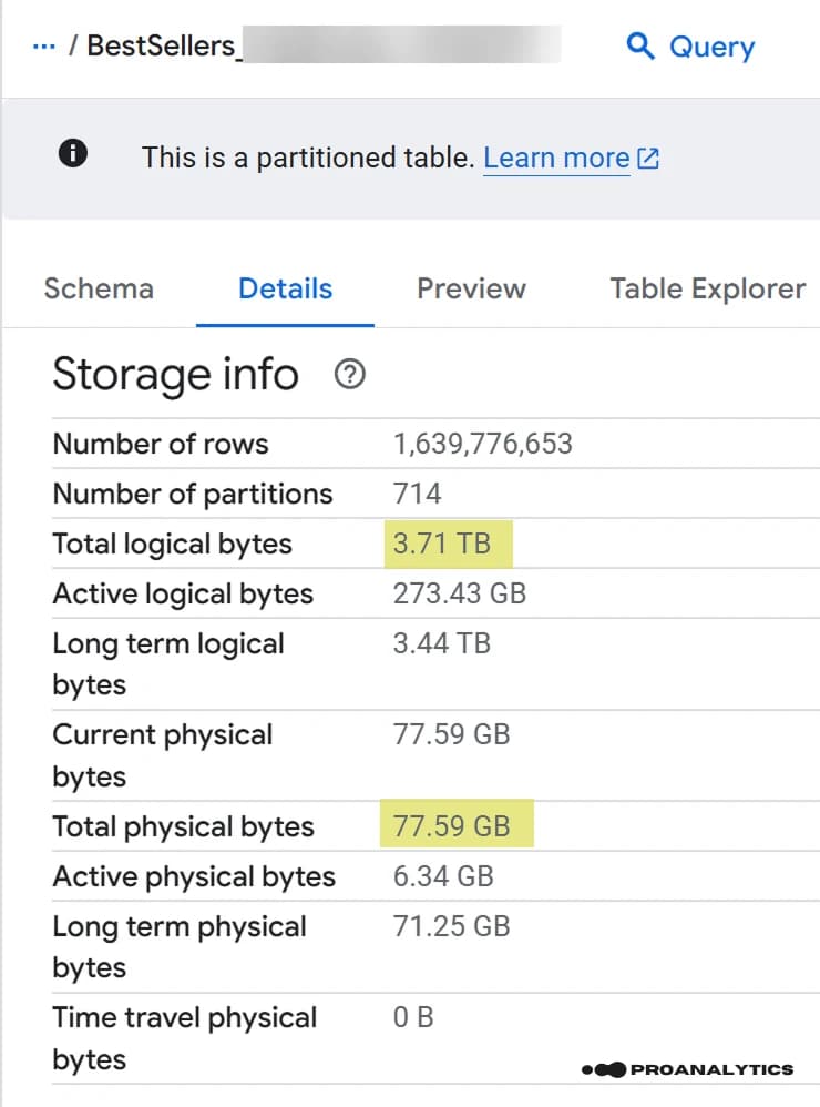
In this article, I want to draw your attention to two key lines that directly affect your costs: Total logical bytes and Total physical bytes, and the difference between them — in this real example, a factor of 49.

Next, we’ll break down what these values mean, what they consist of, and how to work with them.

What’s eating up your budget?

At this stage, we’ll look at two key storage concepts:

Logical vs. physical billing model
Active vs. long-term data storage

Concept 1. Logical vs. Physical Billing Model

Google distinguishes between two storage billing models: logical and physical.
In the first model, you’re charged based on the content of your tables; in the second — based on their actual size after compression.

Let’s use a book analogy:

Logical bytes - the number of characters in the book (pure information).
Physical bytes - the book’s actual weight on the shelf (which can be reduced by changing fonts or using thinner paper).

Imagine you’re buying a book and can choose whether to pay for the number of characters it contains or its physical weight. Naturally, it’s not immediately obvious which option will be cheaper.

We’ll analyze the pros and cons of each model later, but first, let’s look at another important concept.

Concept 2. Active vs. Long-Term Data Storage

Each billing model, in turn, accounts for two types of storage:

Active — tables or table parts that have been modified within the last 90 days.

Long-term — tables or parts that haven’t been changed for more than 90 days (the storage cost for such “old” data automatically drops by roughly half).

Example:

A table was uploaded on April 1 and hasn’t been changed until July 1 (90 days). Starting July 1, it’s classified as Long-Term, and its storage cost is automatically reduced by 50%.

If a table is partitioned, the partitions that are updated or written to remain active, while all others switch to long-term.

Essentially, using partitions is also a way to save on storage without changing the billing model.

How Google calculates your BigQuery storage costs

If you’re already receiving invoices from Google Cloud Platform, you can isolate the specific portion related to data storage.

To view this amount:

Go to your Billing Account Report.
Apply the filter Service = BigQuery.
Group the data by SKU.

Voilà — you’ll now see the familiar lines Long Term Logical Storage and Active Logical Storage. These are exactly the entries that show your data storage costs (by default).

Storage prices may vary slightly depending on your storage region.

For example, here are the storage rates for logical and physical models in Europe:

SKU	Europe (USD / GiB / month)	Comment
Active logical storage	$0.02	The first 10 GiB per month are free.
Long-term logical storage	$0.01	The first 10 GiB per month are free.
Active physical storage	$0.044	The first 10 GiB per month are free.
Long-term physical storage	$0.022	The first 10 GiB per month are free.

Now it’s time to return to the screenshot with the real table example:

Let’s take our data volumes from the screenshot and calculate the storage costs for the Europe region. Here’s the result we got:

SKU	Volume	Europe (USD / GiB / month)	Monthly cost (USD)
Active logical storage	273.43 GiB	$0.02	$5.47
Long-term logical storage	3.44 TB	$0.01	$35.23
Active physical storage	6.34 GiB	$0.044	$0.28
Long-term physical storage	71.25 GiB	$0.022	$1.57

Note: the calculation was made without taking into account the first 10 GiB of free storage.

Let’s sum it up: as a result, the same table can cost roughly $40 per month (if billed for logical bytes — $5.47 + $35.23) or about $2 (if using the physical model — $0.28 + $1.57).

That’s a 20x difference.

And this is just one table. In large projects, we often work with dozens of tables, so the difference between billing models can become quite significant.

Bulk analysis of data volumes within a project

Of course, you could check each table manually to determine its size — but to save time, it’s better to use a query that outputs the necessary information for each dataset.

In this case, I didn’t reinvent the wheel — I took a script from Google’s documentation and just slightly adjusted the output.

Here’s the actual script you need to run in your BigQuery project:

sql

-- Specify the storage prices for your region for the following 4 variables:
DECLARE active_logical_gib_price        FLOAT64 DEFAULT 0.02;
DECLARE long_term_logical_gib_price     FLOAT64 DEFAULT 0.01;
DECLARE active_physical_gib_price       FLOAT64 DEFAULT 0.044;
DECLARE long_term_physical_gib_price    FLOAT64 DEFAULT 0.022;
 
 
 
 
WITH
  storage_sizes AS (
    SELECT
      table_schema AS dataset_name,
 
 
      -- Logical
      SUM(IF(deleted = FALSE, active_logical_bytes, 0))                / POW(1024, 3) AS active_logical_gib,
      SUM(IF(deleted = FALSE, long_term_logical_bytes, 0))             / POW(1024, 3) AS long_term_logical_gib,
 
 
      -- Physical
      SUM(active_physical_bytes)                                       / POW(1024, 3) AS active_physical_gib,
      SUM(active_physical_bytes - time_travel_physical_bytes)          / POW(1024, 3) AS active_no_tt_physical_gib,
      SUM(long_term_physical_bytes)                                    / POW(1024, 3) AS long_term_physical_gib,
 
 
      -- Restorable (these still cost money as active physical)
      SUM(time_travel_physical_bytes)                                  / POW(1024, 3) AS time_travel_physical_gib,
      SUM(fail_safe_physical_bytes)                                    / POW(1024, 3) AS fail_safe_physical_gib
    FROM
      `region-eu`.INFORMATION_SCHEMA.TABLE_STORAGE_BY_PROJECT -- change "eu" to your project region; everything else remains unchanged
    WHERE
      total_physical_bytes + fail_safe_physical_bytes > 0
      AND table_type = 'BASE TABLE'
    GROUP BY 1
  ),
 
 
 
 
  cost_calc AS (
    SELECT
      dataset_name,
 
 
      -- active + long-term Logical
      (active_logical_gib     * active_logical_gib_price)                        AS active_logical_cost,
      (long_term_logical_gib  * long_term_logical_gib_price)                     AS long_term_logical_cost,
      -- active + long-term Physical
      ((active_no_tt_physical_gib + time_travel_physical_gib + fail_safe_physical_gib)
          * active_physical_gib_price)                                           AS active_physical_cost,
      (long_term_physical_gib * long_term_physical_gib_price)                    AS long_term_physical_cost
    FROM storage_sizes
  )
 
 
 
 
SELECT
  dataset_name,
  -- total for logical model (active + long-term)
  ROUND(active_logical_cost + long_term_logical_cost, 2)
                                       AS forecast_total_logical_cost,
 
 
  -- total for physical model (active + long-term)
  ROUND(active_physical_cost + long_term_physical_cost, 2)
                                       AS forecast_total_physical_cost,
 
 
  -- difference logical - physical (positive = logical is more expensive)
  ROUND(
    (active_logical_cost + long_term_logical_cost)
    - (active_physical_cost + long_term_physical_cost),
    2
  )                                    AS forecast_total_cost_difference,
 
 
  -- recommended storage model
  CASE
    WHEN
        ROUND(active_logical_cost + long_term_logical_cost, 2) >0.01
        AND ROUND(active_physical_cost + long_term_physical_cost, 2) <0.01
        THEN 'PHYSICAL'
    WHEN
    ROUND(  (active_logical_cost + long_term_logical_cost)
    - (active_physical_cost + long_term_physical_cost),
    2
  )/NULLIF( ROUND(active_physical_cost + long_term_physical_cost, 2),0)
 
 
   > 2
    THEN 'PHYSICAL'
    ELSE 'LOGICAL'
  END AS recommended_storage_model,
 
 
FROM cost_calc
ORDER BY
  -- sort by datasets where active storage is currently more expensive
  (active_logical_cost + active_physical_cost) DESC;

Note: the calculation was made without taking into account the first 10 GiB of free storage.

To make this query return results, you must have BigQuery Metadata Viewer access. Even a general Owner role won’t provide this information — you need to explicitly add this specific role.

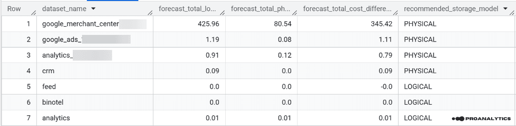
As a result of this query, you’ll get a table with the following columns:

Dataset name
Estimated cost for logical bytes
Estimated cost for physical bytes
Cost difference between billing models
Recommended storage model for each dataset

8.4 Estimated BigQuery storage cost by dataset

The recommended storage model is based on the cost difference and suggests switching to PHYSICAL in cases where the logical cost is more than 2× higher than the physical one.

The 2× threshold is intentional — it reflects the average cost difference between the logical and physical storage models in BigQuery.

Switching to the Physical Model

The next step, based on the results of your table, is to update the datasets where the recommended model is PHYSICAL.

There are several ways to do this, but I’ll show two of the simplest ones.

Method 1. Through the BigQuery Console

Click on the dataset you want to switch to the physical model.
Go to the Details tab.
Click Edit details.
Expand Advanced options.
In the dropdown menu Storage Billing Model, select PHYSICAL.
Click Save.

Method 2. Using an SQL Query

sql

ALTER SCHEMA DATASET_NAME
SET OPTIONS(
storage_billing_model = 'physical'
);

In the query, you’ll need to replace DATASET_NAME with the name of your dataset (for each one you want to change).

I recommend checking your billing account a few days after making these adjustments to see how your data storage costs have changed.

If you’ve done everything correctly, the numbers should pleasantly surprise you.

You might not notice a major difference in your invoices right away, but this is still a step toward cost optimization — one that can save you a significant amount over time.

Results on Real Projects

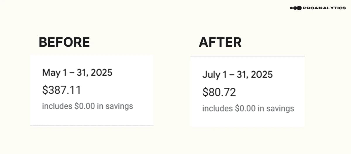
Earlier, I already used data from this project as an example, but I’ll repeat the storage cost results once more — a difference of over $300 per month.

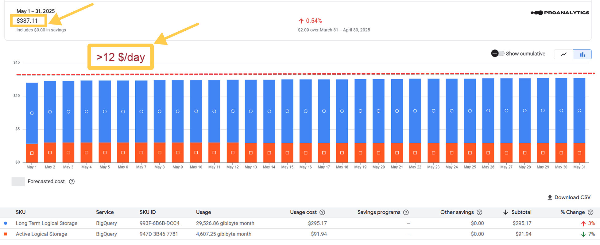
I’ll also add the billing account data before the adjustments (May 2025):

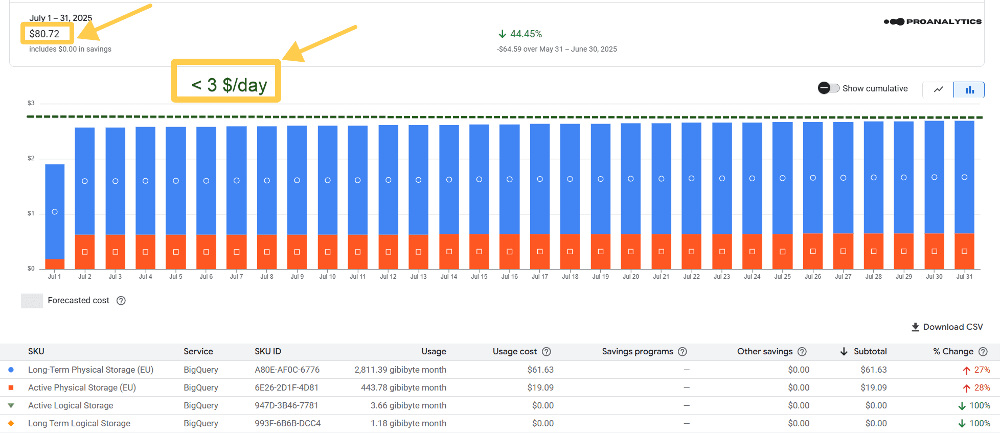
Screenshot for the full month after the adjustments (July 2025):

Before: $387.11

After: $80.72

Savings — over $300/month, i.e. more than $3,600/year.

In this example, I didn’t include a screenshot for June, since we switched to the physical model in mid-June. As a result, the change was only partially visible (for the second half of the month). That’s why I showed the difference using data from the first full month after the switch — July.

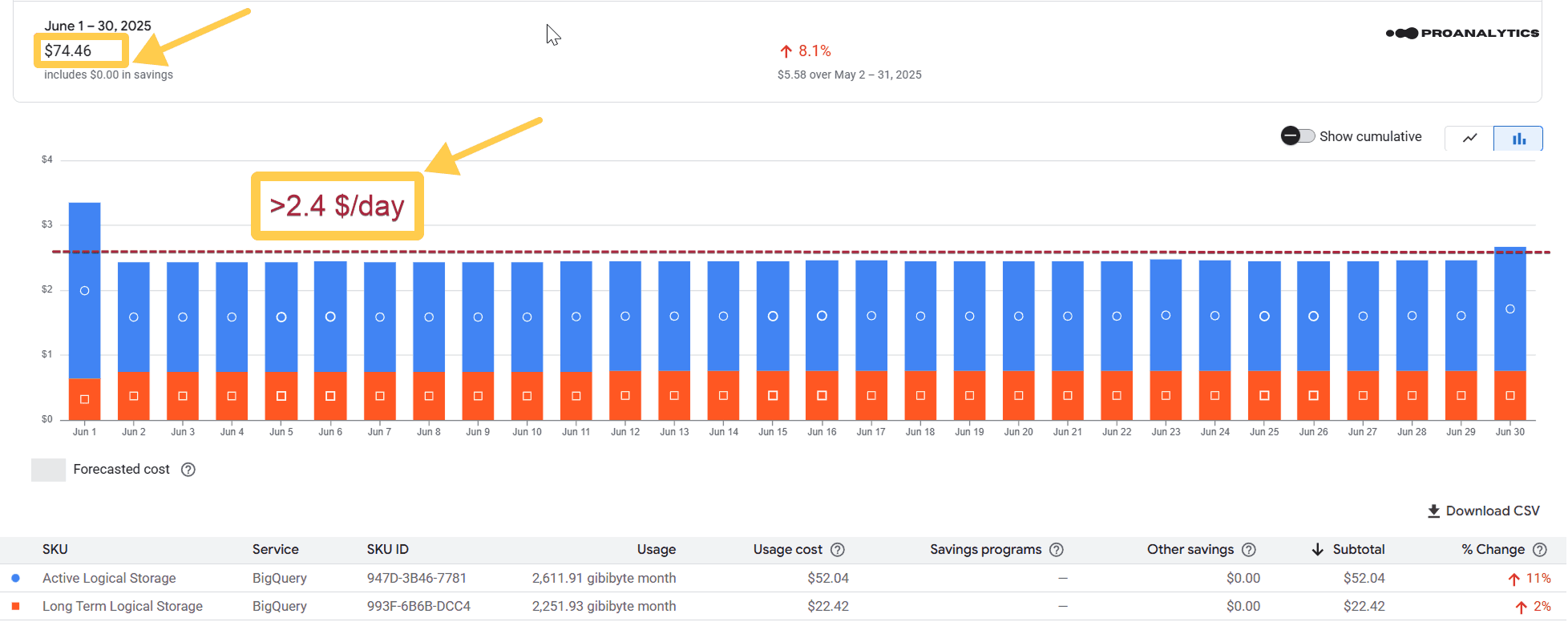
To show that this isn’t an isolated case, here’s an example from another project:

Before the adjustment (June 2025).

After the adjustment (August 2025).

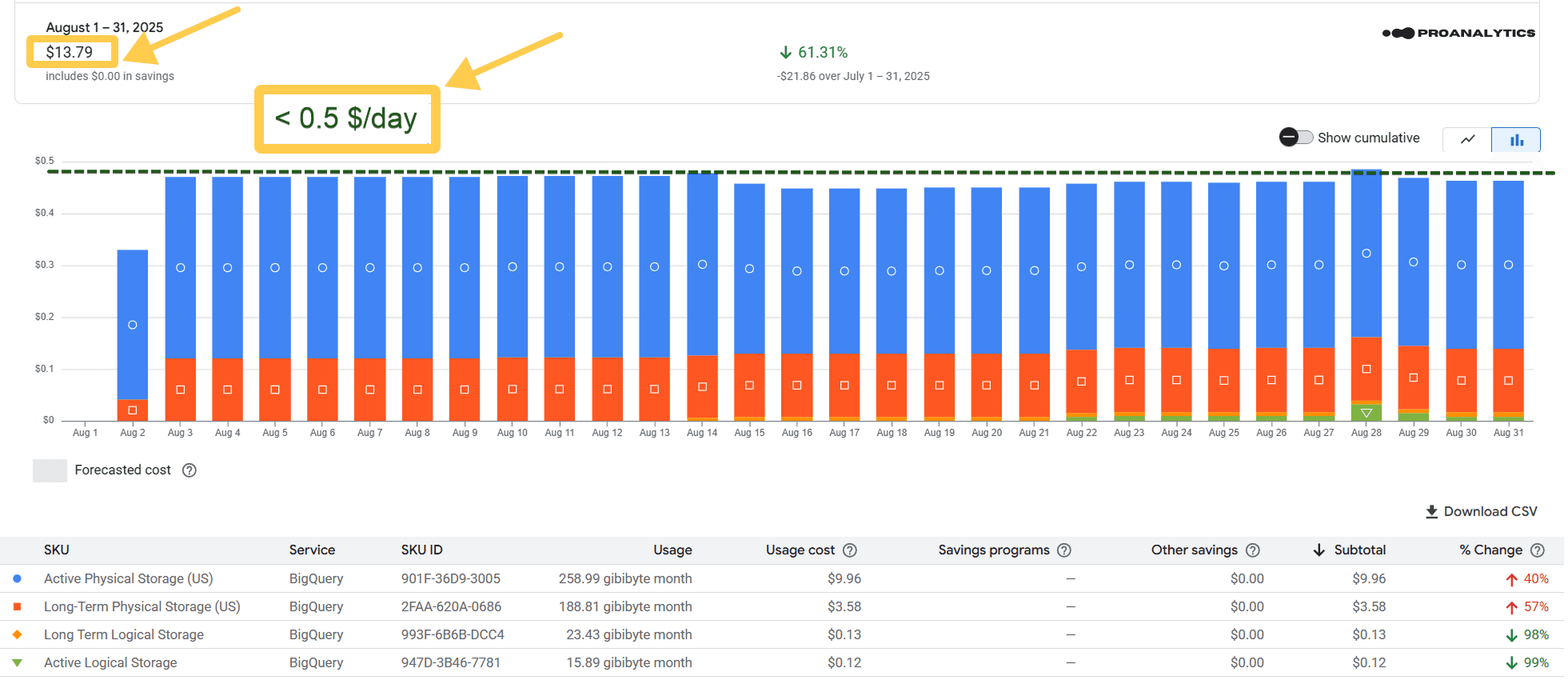
In this example, I’m not including a screenshot for July because we switched to the physical model in mid-July. Accordingly, the result is only partially visible (for the second half of the month). That’s why I showed the changes using data from the first full month after the switch — August.

Before: $74.46

After: $13.79

Savings — over $60/month, more than $720/year.

I’m not sure anything else needs to be said — the numbers, as always, speak for themselves.

What to know before switching

It might seem like there’s a catch — but there isn’t. Google describes this exact billing logic in its documentation, and any user can take advantage of it. It’s a great reminder to read help articles straight from the source.

However, there are a few technical nuances worth noting:

You can change the Storage Billing Model only at the dataset level (not at the table level). That’s why our SQL query also displays data by dataset.
By default, all datasets in your project are set to STORAGE_BILLING_MODEL_UNSPECIFIED, but in reality, you’re already paying for logical bytes (the same LOGICAL model).
If you switch to the physical model and later decide to switch back, you can do so — but only 14 days after the change.
And one more reminder: to make the SQL query from this article work, you need a specific access level — BigQuery Metadata Viewer.

Switching to the physical model is one of the simplest ways to optimize your BigQuery costs without any risks and without changing your data workflow. The difference might seem small at first, but across several months or dozens of tables, it adds up to a significant amount.

Simply put, it’s “smart saving” — an optimization that Google itself offers; it’s just that not everyone has discovered it yet. And of course, this isn’t the only way to save in BigQuery.

If you want to pay less — feel free to reach out ;)

Basic
Google BigQuery
Data Storage
SQL